Site Tools
User Tools
This is an old revision of the document!
Table of Contents
![]()
Installation
Windows
The installation of ToolMap is rather simple. First you have to download the windows installer. It can be found on our web site:
http://www.crealp.ch/fr/accueil/thematiques/cartographie/toolmap/telechargement.html.
The setup wizard will then guide you through the installation process.
Once you have activated the next step, the wizard will generate a default destination folder for the installation; you can, of course, change the destination folder.
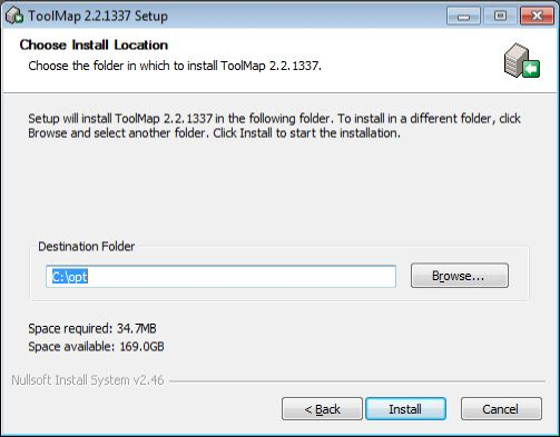
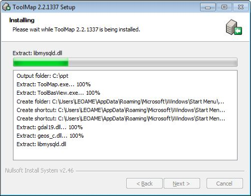
If you click on the [install] button, the installation will begin. Otherwise you can go back to change settings or simply cancel the operation. If you decided to launch the installation, a progress window will pop up. The installation process should be pretty fast.
Once the installation has been completed you'll have the choice to create a desktop shortcut before closing the setup wizard.
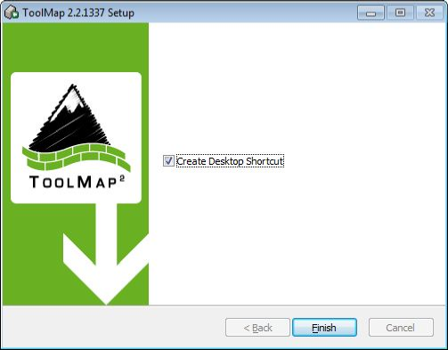
ToolMap can now be launched using either the desktop icon or the menu entry located in Programs → ToolMap2 → ToolMap
Silent Installation
ToolMap may also be installed without requiring the user to select options or click next. This mode, also called unattended installation, may be particularly useful for system administrator trying to deploy ToolMap on multiple computers without the hassle to go through all the wizard pages.
Installing
The following command line may be used for the silent installation of ToolMap:
InstallToolMap_d967.exe /S /INSTDIR=”C:\Program Files\ToolMap2” /AllUsers
- /S: inform the installer to be silent
- /INSTDIR: Path for installing ToolMap
- /AllUsers (or /CurrentUser): Install ToolMap for all users (administrator privilege required) or for the current one only.
Uninstalling
The following command line may be used for uninstalling ToolMap silently:
“C:\Program File\ToolMap2\uninst.exe” /S
Mac OSX
Download the ToolMap’s .DMG file from http://www.crealp.ch/fr/toolmap-telechargement.html and then double-click on it. A new Finder window similar to the one illustrated bellow should appear.
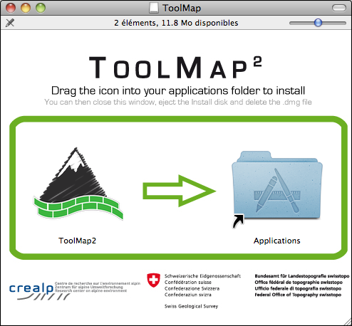
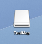
Drag the ToolMap icon into the “Applications” folder to install ToolMap. Once ToolMap is installed, you can safely eject it's disk image. Click on the ToolMap disk icon on the Desktop and then press CMD-E.
Delete the .DMG file by dragging it to the trash.
Linux
ToolMap is actually only available as Debian (*.DEB) package for Ubuntu. To install ToolMap, you may either run the following command line: sudo dpkg -i toolmap_2.4.1337_amd64.deb or use your favorite package manager
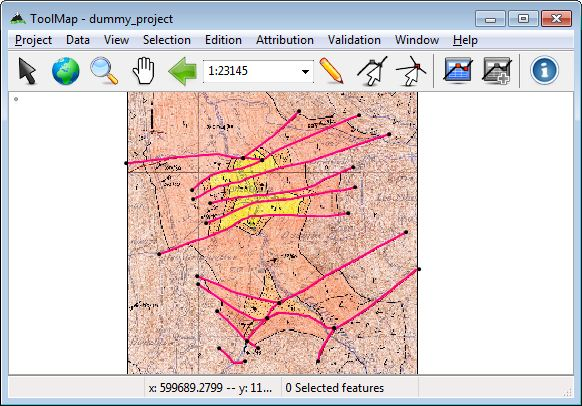
User Interface Overview
The ToolMap user interface integrates the following elements:
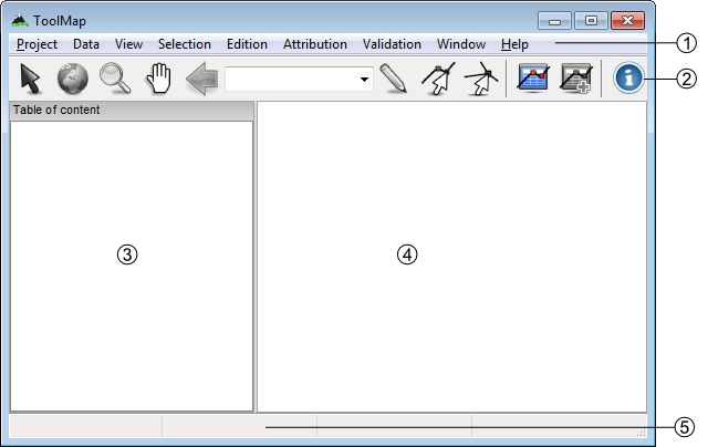
- Menu bar
- Toolbar
- Table of content
- Visualization and editing window
- Status bar
Menu bar
In the menu bar nine menus are available, each of them will lead you to different options:
- Project: This menu contains all options related to the project management.
- Data: This menu allows the user to add or import support data into the project.
- View: The view menu contains all options for navigating and zooming into the displayed data.
- Selection: This menu contains tools for managing the selection.
- Edition: All tools related to the editing process are located into this menu.
- Attribution: This menu contains the tools used when attributing datas.
- Validation: This menu contains the tools used to check the objects and layers before exportation as well as the Statistics… tool.
- Window: windows management and other functionalities.
- Help: The Help Menu provides various help functions as well as options for reporting a bug.
Toolbar
The toolbar is accessible on top of the application window, right under the menu bar. It allows to quickly access to the different main tools available in ToolMap. Most of the toolbar buttons are grayed out while no project is open.
Selection tool
 Select one or several geometrical objects
Navigation tools
 Zoom to the maximum extent of all visible layers
 Zoom in or out into the visualization window
 Pan the view in any direction
 Go back to the previous zoom extent
Edition tool
 Draw a new object
 Modify an existing object
 Modify shared node
Attribution tools
 Display the Object kind panel
 Display the Object attribute window
Information tool
 Display the identification window
Scale
 Drop-down menu of available scales. User defined scale can be set using the Project → Edit → Settings menu
Table of Content
The table of content shows a list of all the layers loaded in the project. It looks like the following:
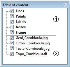
- Construction layers, they are automatically generated at the creation of the project and can be edited. They are displayed using a bold font.
- Support Themes, they cannot be edited.
Status bar
The status bar at the bottom of the application window provides additional information like geographical coordinates or the number of features selected.
Keyboard shortcuts
Keyboard Shortcuts have been set to the most used functions to make the use of Toolmap easier and quicker.
Project management
- Ctrl+N: Create a new empty project
- Ctrl+Alt+N: Create a new project based on a template
- Ctrl+Alt+O: Open an existing project
- Ctrl+S: Backup the project
- Ctrl+Alt+S: Save the project as a template
- Ctrl+Alt+E: Open the export layer window
- Ctrl+O: Link data
- Ctrl+W: Unlink data
Navigation tools
- <: Previous zoom
- Z: Zoom tool
- H: Pan tool
- Ctrl+0: Zoom to the full extent
- Ctrl+1: Zoom to frame
- Ctrl+2: Zoom to selected layer
- Ctrl+R: Refresh display
Editor tools
- D: Draw a feature
- M: Modify a feature
- P: Draw a Bezier
- A: Modify a Bezier
- Ctrl+Z: Remove the last vertex
- Ctrl+V: Display the vertex positions window
- I: Insert vertex
- C: Delete vertex
- Ctrl+T: Move a shared Node
- DEL: Delete the selected objects
- Ctrl+X: Activate the line cutter tool
- Ctrl+F: Merge the selected lines
- Ctrl+I: Create intersections
- Ctrl+Alt+F: Flip the selected line (change the orientation)
- Ctrl+G: Display the snapping panel
- Ctrl+Alt+G: Display snapping radius
- V: Selection tool
- Ctrl+D: Clear Selection
- ENTER OR TAB: Finish a segment or apply the modifications
- ESC: Cancel an edition or modification
Attribute tools
- Ctrl+A: Display the Object attribute window
- Ctrl+Alt+A: Display the Object attribute window (batch)
- Ctrl+Y: Set Orientation tool
Others
- Ctrl+L: Display the log window
- Ctrl+Alt+R: Run the selected query
- Ctrl+Alt+I: Display the information Window
Project Management
The whole management of the project is made with the menu Project, which includes the following options:
- New Project: create a new project
- Open…: open an existing project
- Recent: open a recently used project
- Backup: create a backup of the project
- Manage backup: open the backup management window
- Save as Template: save your project as a template
- Export Layer…: export a layer or the project as shapefile
- Export Model as PDF…: export your data model as PDF
- Edit: edit the project
- Exit: quit ToolMap
New project
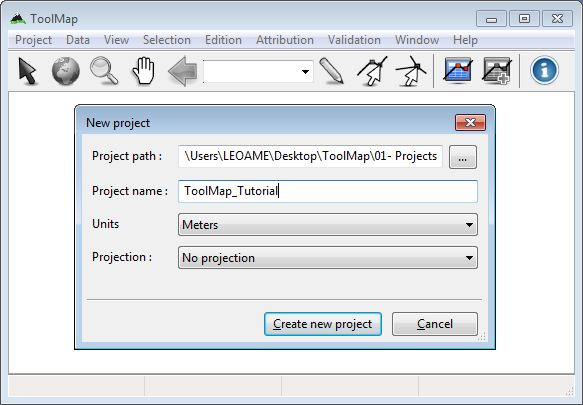
To create a new project, select Project → New Project → Empty…. The dialog box illustrated bellow appears.
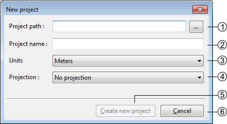
- Project Path
- Project name
- Units (meters, Kilometers, Lat/Long). Actually this option isn't enabled and projects are always using meters as their units
- Projection system (no projection, Swiss projection). Actually this option isn't enabled and only “no projection” is supported.
- Create a new empty project and activate the next step
- Cancel the creation of the project
Generalities
The Project Properties tab of the Project Definition window allows to complete some generic project information.
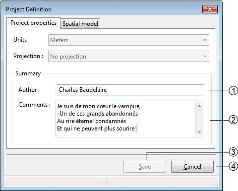
- Define the author of the project
- Comments about the project
- Saves the properties modifications of the project (this button is enabled only when at least one layer is created)
- Cancel the properties modifications of the project
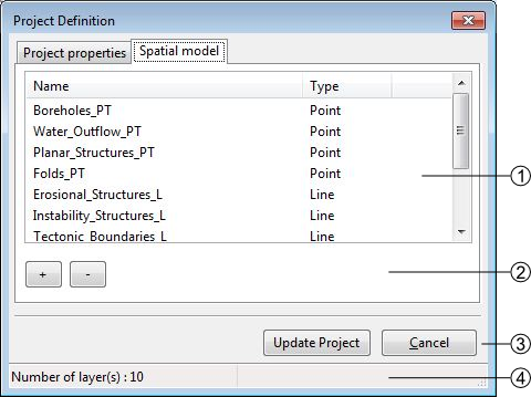
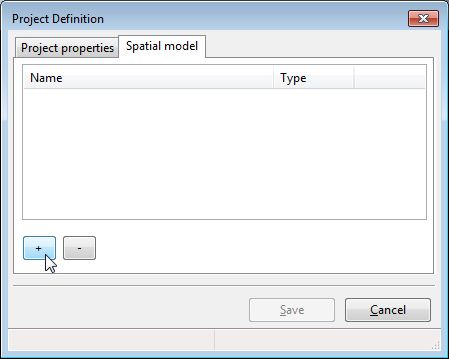
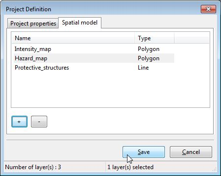
Spatial model
The Spatial Model tab of the Project Definition window lists the layers. Each layer contains objects and may have attributes.
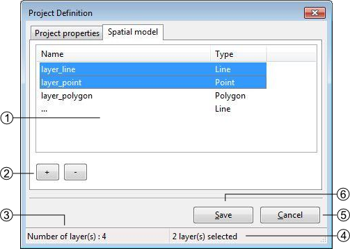
- List of layers defining the spatial model, several operations can be realized in this list:
- Editing the characteristics of a layer by double-clicking on it
- Sorting layers by clicking on the list header
- Reorganizing layers order with a contextual menu
- Layers management controls
- [+]: add a layer
- [-]: delete one or several selected layer(s), the suppression can also be made with the DELETE or BACKSPACE keys.
- Number of layers
- Number of selected layers
- Save the project modifications (this button activate only when at least one layer is created)
- Close the window without saving the modifications.
Layers Definition
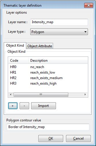
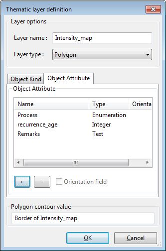
The Thematic layer definition window appears when adding a new layer:
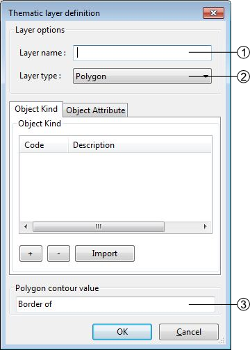
- Layers name. This name is used as the output file name when exporting the layer.
- Spatial layer type (line, point, polygon)
- Name of the polygon contour. This field is only displayed for polygon layers
Object kind definition
The objects belonging to a layer are defined in the Object kind tab of the Thematic layer Definition window
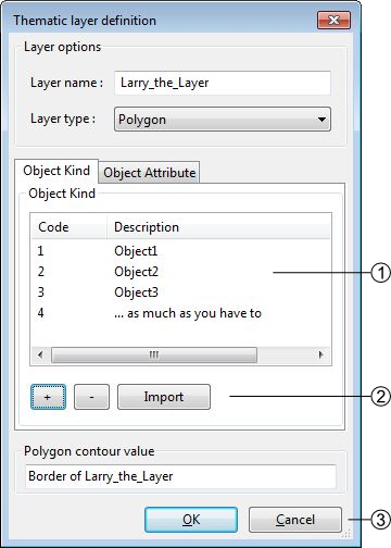
- List of defined objects. Following operations can be realized in the list:
- Sorting objects by clicking on the list header
- Editing the objects characteristics by double-clicking on an object
- Reorganizing objects order with a contextual menu
- Objects management controls
- [+]: Add an object
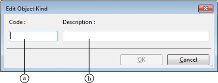
- Code (numerical value) duplicates are allowed but not recommended. This code will be exported as OBJ_CD field when the layer is exported
- Description: a textual description of the object. This value will be exported as OBJ_DESC field when the layer is exported
- [-]: Delete one or several selected objects. The suppression can also be made with the DELETE or BACKSPACE keys.
- [Import]: import list of objects from files of following format:
- *.CSV Format :<Code>;<Description>;<Theme>;<Frequency>
- *.TXT Format :<Code>[TAB]<Description>[TAB]<Theme>[TAB]<Frequency>
- Save or cancel the object modifications
Attributes definition
The attributes management is made from the Attributes tab of the Thematic layer definition window.

- List of defined attributes
Following operations can be realized in the list:- Sort attributes in alphabetical order by clicking on the Name or Type header
- Edit an attribute characteristic by double-clicking on it
- Reorganize the list of attributes with the contextual menu by right-clicking
- Attributes management controls
- [+]: Add an attribute
- [-]: Delete one or several pre selected attributes. The suppression can also be made with the DELETE or BACKSPACE keys.
- Save or cancel the attributes modifications. An attribute is defined by:
- A name: the name cannot contain spaces or reserved words (annexe)
- A type of data:
- Text
- Integer
- Float
- Date
- Enumeration
Attribute creation
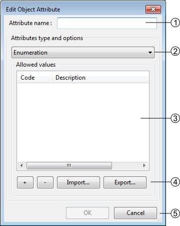
- Attribute name
- Attribute type
- Attribute options: each type has different options, in this case the enumeration type. Following operations can be realized in the list:
- Sort the values of the list by alphabetical order by clicking on the Code or Description header
- Edit values characteristics of the list by double-clicking on it
- Reorganize the list of values with the contextual menu by right-clicking
- Enumeration management controls
- [+]: add a new value
- [-]: delete one or several pre selected values. The suppression can also be made with the DELETE or BACKSPACE keys.
- [Import]: import lists of values, two types of format can be imported:
- *.CSV Format: <CODE>;<Description>
- *.TXT Format: <CODE>[TAB]<Description>
- [Export]: export the list of values in TXT files
- Save or cancel the list of values modifications.
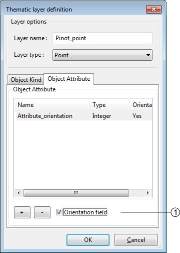
Orientation of a point type object
It's possible to orientate an object of a layer. However, several constraints have to be considered:
- The spatial type of the layer has to be a Point type
- The data attribute type has to be a Float or an Integer type
- Only one attribute per Layer can be oriented.
Activation of the orientation
In the Object Attribute tab of the Thematic layer definition window, you have to select the attribute by clicking on it, and then activate the case Orientation Field at the bottom of the window(1)(see also attribute orientation to point for further information).
Create from template
The option Project → New Project → From template… allows you to create a new project with the same layers/objects/attribute as an existing one. This option will create a new project from an existing template. The creation is made through the two following steps:
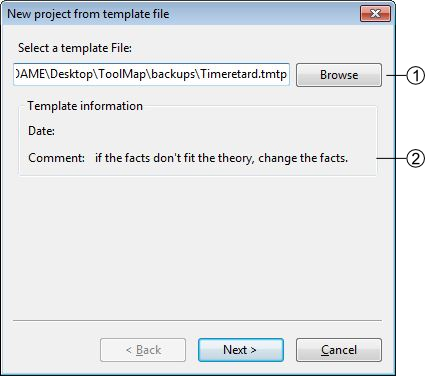
- existing template path
- Template information
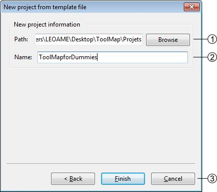
- Directory for the new project
- Name of the new Project
- Creation controls:
- Back: Return to the previous window (choose another template)
- Finish: Create the new project with the current settings
- Cancel: Cancel the creation of the new project
Open a project
There are two possibilities to open an existing project:
- With the option Project → Open…: open a project saved on your computer
- With the option Project → Recent: open a project which had already been opened recently
Special cases
- The project do no more exists, it was whether deleted or moved.
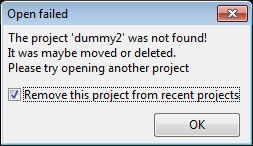
- If the box is checked it will automatically erase the project from the list of the recent projects.
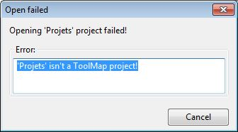
- The folder you selected is not a ToolMap file
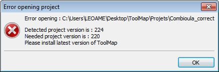
- The project was made on an older version of ToolMap and need to be upgraded
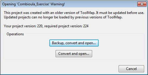
- The backup and convert option generates a backup of your project in the old version of ToolMap and upgrade the current project
- The convert only option simply converts the version of your project. Be aware that your project will no more be readable by older version of ToolMap.
Edit a Project
The Edit option from the menu Project allows editing the characteristics and components (layers, objects, attributes, settings) of the current project.
Edit the project properties
The layers and attributes of the project can be modified with the Project Definition…function of the Edit submenu.
The first tab Project Properties of the window allows modifying the properties of the project like the name of author and the eventual comments. (See chap. Generalities)
The second Tab Spatial Model allows modifying the layers (see chap. Spatial model) and the attributes (see chap. Attributes definition).
Edit objects
The objects can be modified with the menu Project→Edit→Objects kind… They are distributed in the three spatial kinds: point, line and polygon.
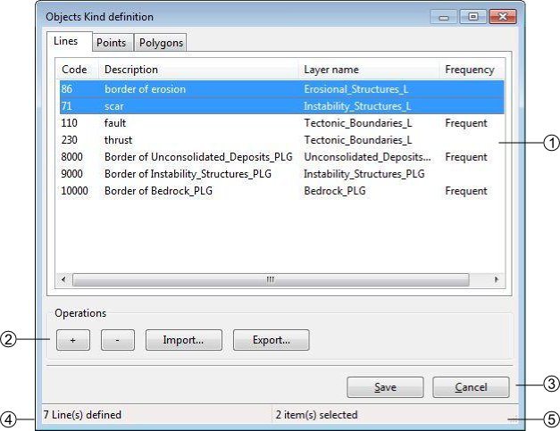
- List of objects defined by spatial type. Following operations can be realized in the list:
- Sort objects by alphabetical order by clicking on the Code, Description, Layer or Frequency header.
- Edit the objects characteristics by double-clicking on it.
- Reorganize the list of objects with the contextual menu by right-clicking.
- Objects kind management controls
- [+]: add an object
- [-]: remove the selected object
- [import]: import an object
- [export]: export the selected object
- Save or cancel the objects modifications
- Number of objects in the selected spatial type
- Number of selected objects
Edit attributes
The attributes can be modified with the option Project→Edit→Object Attribute…
- List of available layers, you can modify them by double-clicking on it
- Objects management controls
- [+]:add a new layer
- [-]: delete the selected layer
- [Update]: update the project saving the modifications
[Cancel]: Cancel the modifications - Number of available Layers
Settings
The settings edition is activated with the option Project → Edit → Settings…
Project Settings
The project settings tab of the project settings window allows to manage the export and backup properties
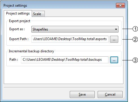
- Export data type (Shapefile, Graphics (EPS))
- Export file path
- Backup file directory
Scale
The scale tab of the project settings window allows managing the scales

- List of defined scales. Following operations can be realized in the list:
- Edit a scale by double-clicking on it
- reorganize the list of scales with the contextual menu
- Scales management
- [+]: Add a new scale
- [-]: Delete one or several preselected scales. The suppression can also be made with the [Delete] or [Backspace] keys
- Management options of the scales list. The list can be ordered with the options of the order drop-down menu
- Sort ascending
- Sort descending
- User defined: ordered by the user
- Save or cancel the settings modifications
Save and restore a project
Backup
When working on ToolMap the changes are automatically and constantly saved. Because of that it is safe to create frequent backups of the project. The Backup function from the menu Project allows you to make backups of your current project.
At the creation of a backup, you can write a comment about your save.
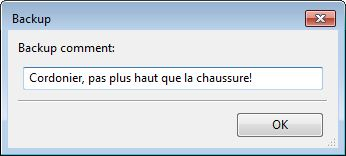
The comment will appear in the Manage Backup window.
The Manage Backup window is accessible with the option Manage backup from the menu Project. This window lists all the backups stored in your backup file. The name of the backups is automatically generated following this model: Projectname-YYYY-MM-DD-HHMMSS
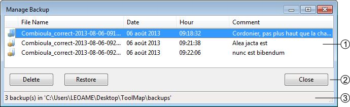
- List of the backups with their characteristics and comment. The list can be ordred by each of the characteristics
- Backups management controls
- Delete: Delete the selected backup(s)
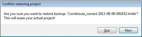
- Restore: Restore the selected backup. When clicking on this option, a window asks you the confirmation of the restoration process.
- Close: Close the window and return to your current project
- The Backup path (beforehand defined in the Settings)
Template
You can create templates of your project with the option Save as template… from the menu Project. The creation of a template is made as such:
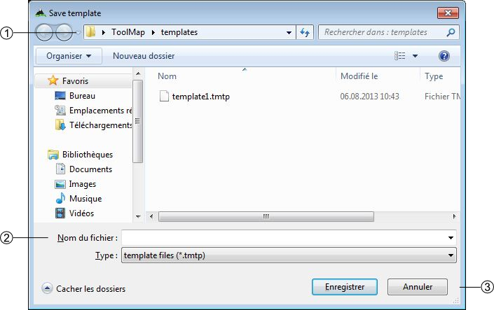
- Path where the template will be stored
- Name of the template and the format
- Save the template or cancel the operation
After saving your template you can enter a comment that will appear if you use the create from template option.
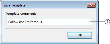
- Comment on the template
Export a project
Export Layers
The exportation allows generating layers, which were defined at the spatial model level in order to be used in others programs. The export path and format have to be beforehand defined (see chap. Settings)
The exportation is made with the option Export Layer… from the menu Project. When selecting this option the following window appears:
- List of the layers defined in your data model
- Layers selection controls
- All: select all the layers
- None: remove all the selected layers
- Invert: invert your current selection
- Export or cancel the exportation
When Exporting a Polygon Layer, ToolMap automatically create a column “NB_LABELS” in the resulting file. This column is filled for each polygon with the number of labels inside that polygon.
Export Model as PDF
Once the spatial model of a project is set, you can get a PDF layout of it using the Export Model as PDF tool (Project→Export→Export Model as PDF…).
The following window will then open :

- Choose to either print your data model on a single page or with one layer only per page. The later allows you to choose between several paper sizes (from A0 to A4) and orientation (Portrait or Landscape).
- Choose the layout of your data. The upper option will display Object Attributes below the Objects Kinds, the lower option will display them next to each other.
Checking the “use very simple decorations” box in the next window will allow you to print a lighter version of the document.
Close the Project
To quit the project, you just have to click on the upper-right icon or select the option Project → Exit.
Spatial Data management
The data management is made through the Data menu, it contains the following elements:
- Link data… (Ctrl+O): reference a support layer which will be displayed in your project
- Unlink data… (Ctrl+W): unlink a layer
- Import data: import data into one of your construction theme
Link data
The Link Data… option from the menu Data allows loading some support themes for the vectorization of the construction layers. Those support themes can be vector data (*.shp) or raster data (*.tif, *.JPG and Esri's binary GRID).
In the opposite of the construction layers, the support themes are not stocked in the project but only referenced.
Rotation
Some of your files may have rotation information, which is not yet supported by ToolMap. In that case you will see the following message:

- rotation information
- display option
This message will pop up every time you make an action regarding the layer (including trivial actions like zoom or pan), so be sure to convert your images into non-rotated rasters. If the rotation is insignificant, you may prefer to simply ignore the message by checking the option Hide warnings for this layer. This option prevent the appearance of the message for the current session, but it will pop again the next time you launch your project.
Import data
The Import data… option from the menu Data allows you to import some existing information into your construction layers. You can only import lines or points geometries. The process is made in 3 different steps.
Step1

- the Import data… option allows two types of data, choose the one you want to import
- Go to the next step of the import or cancel the operation
Step2
If you choose to add a shapefile the following step comes ahead

- Directory path of the shapefile
- data information of the shapefile
If you choose to add a CSV file the following step comes ahead

- Directory path of the CSV file
- Information on the CSV file
- allow to go back or to continue to step 2.2
Step2.2
The CSV files are composed of columns of data separated with commas, you will have to choose wich column you want to assign to the X and Y coordinates

- List of the columns which can be assigned as X or Y coordinates
- allows to go back or to continue to step 3
Step3

- List of layers within the data will be imported (with the shapefile import the choice is restricted to the geometrical type of the data)
- import the data or cancel the operation
Table of contents options

 : Activate the display of the layer
 : Deactivate the display of the layer
- Edition mode activated: the layer is underlined
contextual menu
The contextual menus are opened by right-clicking on a layer of the table of contents. They vary according to the selected layer.


- Name of the layer
- Edit this layer(construction layers only)
Remove layer(support themes only)
- Move the selected layer in the table of contents

- Display management of the vertex (line and polygon layers type only)
- Symbology management. This option can also be activated by double-clicking on the layer. (see chap. Symbology)
Visualization
The different tools allowing you to explore your project in the visualization window are stored in the View menu, it regroups the following elements:
- Previous zoom (<): go back to the previous displayed scale, available only if you have once changed the scale
- Zoom by rectangle (Z): This tool uses a click-release action, click on the left button of the mouse and drag it, it makes a rectangular ghost. The zoom factor is inversely proportional to the size of the rectangle. The type of zoom is determined by the direction of the drag:
- Left to right: zoom in
- Right to left: zoom out
- Pan (H): Move the map with a drag and drop action
- Zoom to full extend (Ctrl+0): Adjust the scale to display all the activated layers
- Zoom to frame (Ctrl+1): Adjust the scale to display the frame.
- zoom to layer (Ctrl+2): Adjust the scale to display the whole selected layer
- Refresh (Ctrl+R): Refresh the screen
Symbology
The symbology windows allow you to manage the style of each layer. You have several options available depending of the layer style. They are accessible by double clicking on the layer name in the table of content or with the option Symbology… of the contextual menu.
Points
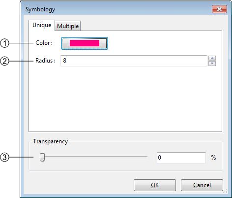
- Points style management: you can change the color and the radius of the points
- Transparency management
- Apply or cancel the modifications
The points have an additional option found on the other tab of the window (multiple). Under this tab you are able to attribute two different symbology to your lines. The differentiation of the points is made through the queries.
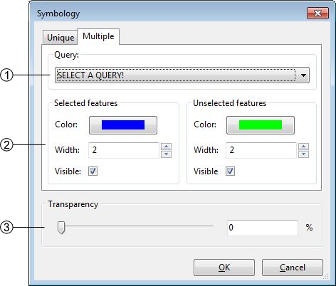
- Query selected for the differentiation
- symbology management of the two classes
- transparency management
The symbology is directly connected to the attribution of the point, changing its attributes may instantly change its symbology. This option can be very helpful to highlight specific classes.
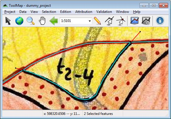
Lines
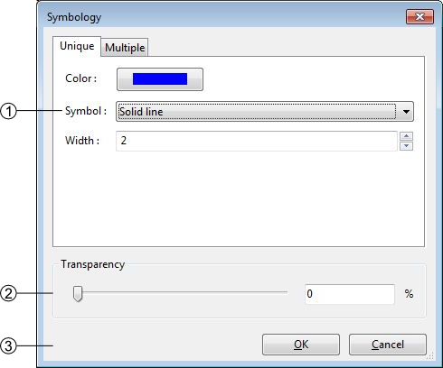
- Lines style management, you can change the color the width and the symbol of the lines. There are six choices of shape. Choices are:
- Solid line
- Dotted line
- Dashed line
- Dot-dashed line
- Transparant line: The Transparent line option may be used to hide the lines.
- Oriented line: The Oriented line option display a double line: solid and dotted side by side. This option can be used to check for consistency when some lines have to be drawn in a certain direction.
- Transparency management
- Apply or cancel the modifications
The lines have an additional option found on the other tab of the window (multiple). Under this tab you are able to attribute two different symbology to your lines. The differentiation of the lines is made through the queries.
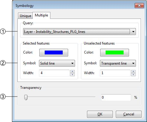
- Query selected for the differenciation
- symbology management of the two classes
- transparency management
The symbology is directly connected to the attribution of the line, changing its attributes may instantly change its symbology. This option can be very helpful to highlight specific structures.
Polygons
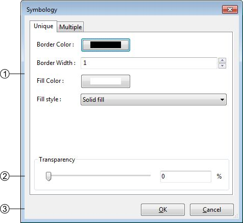
- Polygons style management: you can change the border width and color as the fill color and style. Following styles are available:
- Solid fill
- Backward Diagonal hatch
- Forward Diagonal hatch
- Cross hatch
- Vertical hatch
- No Fill
- Transparency management
- Apply or cancel the modifications
If your imported polygons have attributes, you can class them to have a multiple symbology. (see also Redactor mode)
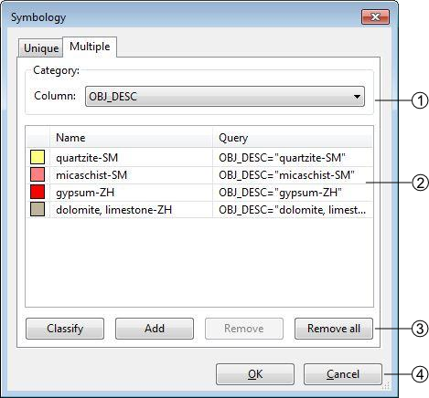
- List of attribute header
- List of the different attributes related to the header
- Symbology controls:
- Classify: Generate the classes depending of your choice in (1)
- Add: Add a new class, you will have to write the query yourself
- Remove: Remove the selected class
- Remove all: Remove all the classes
- Validate or cancel the changes
Images
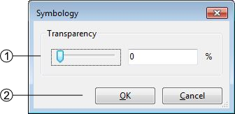
- Transparency management
- Apply or cancel the modifications
Features Selection
The tools allowing you to select features in the visualization window are regrouped in the Selection menu:
- Select (V): select one or more object in the current layer in edition
- Select by Feature ID…: select an object with its ID
- Clear Selection (Ctrl+D): clear the current selection
- Invert Selection: unselect the current selection and select all non selected objects
Single Selection
Regardless you want to make a simple or a multiple selection, you have to be in edition of the correct construction layer to target an object.
You have two ways to select a unique feature:
- By using the selection tool: Activate the selection tool by clicking on it in the toolbar or by selecting it in the menu Selection. Then simply clik on the object you want to select in the visualization window.
- By using the Select by Feature ID… tool: Every object in a ToolMap project has a unique ID, you can also select a precise object if you know its ID.
Multiple Selection
The multiple selection is made with the selection tool. You can either click and drag your cursor to select all the features within the rectangle or by selecting single features one by one maintaining the Shift key.
Edition
All the edition tools are regrouped in the menu Edition, which contains the following elements:
- Draw D
- Modify feature M
- Draw Bezier P
- Modify Bezier A
- Bezier Settings
- Remove last vertex Ctrl+Z
- Edit vertex Ctrl+V
- Insert Vertex I
- Delete Vertex C
- Move shared node Ctrl+T
- Delete feature Delete
- Cut line Ctrl+X
- Merge lines Ctrl+F
- Create interection Ctrl+I
- Flip line Ctrl+Alt+F
- Snapping
Edition tools
To edit objects with the different tools in ToolMap you will have to enter the edition mode.
- Select the layer to edit in the table of contents
- Activate the Edit Layer option in the pull-down menu
This operation activate the edition menu
Draw feature
The draw tool allows creating new features
Point type layer
- Activate the tool, the edition cursor displays
- Vectorize the point with a left click
Line type layer
- Activate the tool, the edition cursor displays
- Vectorize the line with the mouse, each left-click creates a vertex
- Cancel the last vertex of the segment in edition; Remove last vertex(Ctrl+Z) option of the Edition menu
- Finish the construction of the object with the ENTER or TAB key
- Cancel the segment in creation with the ESC key
Modify feature
The modify option allows modifying features.
Point type layer
- Select a point
- Activate the tool ; the modification cursor displays
- Modify the position of your selected point by dragging it with your cursor
Line type layer
- Select a line
- Activate the tool ; the modification cursor displays
- Modify the vertex position with the cursor by dragging it
- Cancel the modification of the current segment with the ESC key
- Apply the modifications with the ENTER or TAB keys
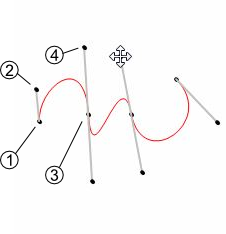
Draw Bezier
The draw Bezier tool allows building Bezier curves. For each section of Bezier you’ll have to click four time(see below).
- Defines your starting point
- Defines the direction of your Bezier at the starting point
- Defines your arriving point
- Defines the direction of your Bezier at your arriving point
Modify Bezier
While drawing your Bezier curves, you can modify them using the option Modify Bezier. This option allows you to move your starting/arriving points also the orientation and intensity of the way.
Bezier Settings
In the Bezier settings you can manage the parameters of the Bezier. You have access to two styles of parameters:
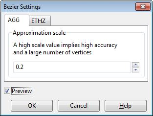
- The AGG fashion: Have only one parameter, the higher your value the more complex your curve (more vertices).
- The ETHZ fashion: With the ETHZ method you can play on two parameters; the maximum number of points for each segment and the width tolerance. While the maximum number is easy to understand the width range defines whether a vertex is created or not, the higher the range, the more simple your curve.
The Preview option displays how the line will be created regarding the parameters. It is only available while drawing a Bezier.
Remove last vertex
While drawing a line or a Bezier, this tool allows you to remove your last vertices. This tool works only during the vectorization process. This tool will not remove vertices from a validated line.
Edit Vertex
Allows modifying the geographical coordinates of the vertices.
- Select a feature
- activate the tool ; The following window pops up
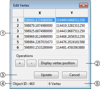
- Geographical coordinates of the vertices defining the geometry of the feature
- The coordinates can be directly edited in the table.
- [+]: add a new Vertex, the insertion is made after the current selection. The X,Y coordinates have to be edited. The insertion of a vertex without coordinates provokes an error message at the update of the geometry ([Update]).
- [-]: suppression of the selected vertex.
- [Display Vertex]: Visualization of the selected vertex.
- Update or cancel the current modifications
- Selected feature ID
- Number of vertices of the selected feature
Insert vertex
This tool allows you to insert vertices on a selected line. To do so activate the tool with the option insert vertex in the edition menu or with the I shortcut and simply click on your selected line where you want an additional vertex.
Delete vertex
The Delete vertex tool allows you to delete any vertices on a selected line. To do so simply activate the tool selecting the option delete vertex in the Edition menu or with the C shortcut and aim for an unwanted vertex, it will be obliterated.
Move shared node
The Move shared Node allows to move a vertex which is assigned to more than one line. The point is to move a vertex by keeping the boundaries of every lines related to it. This tool is activated using the menu Edition→Move shared node(Ctrl+T) or using the corresponding button in the toolbar.
Delete selected feature
allows deleting the selected features
- Select the feature(s)
- Use the option Delete selected feature of the Edit menu or use the Delete or Backspace key
In the case of a multiple selection, a window appears asking a confirmation of the suppression.
Cut line
The cut lines option allows cutting lines. The cut can only be done on a vertex.
- Select a line
- Activate the tool with the menu or with the shortcut (Ctrl+X) ; the tool cursor displays
- click on the vertex where the division must be done
The two lines will then have the attributes of the original line.
Merge Line
Allows merging the selected lines. The selected lines have to be adjacent, the lines must have a begin/end vertex in common.
- Select lines
- Activate the tool : several cases are possible:
- Same attributes ⇒no consequences
- Different attributes ⇒ the user has to define the attributes to keep
- 1 non attributed object ⇒ the user has to define the attributes to keep
- Same polarity ⇒ no consequences
- Different polarities ⇒ the polarity becomes left to right
Create intersection
Allows creating intersections between lines which cross themselves. All the segments created will keep their previous attributes
- Select a line which cross another one.
- Activate the tool with the menu or with the Ctrl+I shortcut.
Flip fline
The Flip line option allows to reverse the polarity of the selected line. To check the polarity of the line you have to either open the vertex editor (see Edit vertex) and check the coordinates of the first vertex or use the Oriented line symbology. The tool can be used on multiple lines at once.
snapping
The snapping tools are accessible via the menu Edition → Snapping
During the vectorization of a point or line feature, the snapping function allows to hang on the nodes of an existing feature. The snapping can be done on the features of the active layer (i.e. current edition) and/or on features belonging to other layers (construction layers and vectorial support themes)
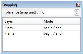
Snapping panel
The snapping panel (Ctrl+G) is defined by the following elements:
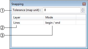
- The capture tolerance of nodes
- The involved layers
- The mode of snapping used for the involved layerlayer. You can choose between :
- None: the snapping is disabled on this layer.
- Begin/end: the snapping occure only on the first and last vertices of a line.
- All vertex: the snapping occure wherever there is a vertex.
Snapping display
Using the option Show snapping radius on map (Ctrl+Alt+G); you will display a circle in the top left corner of the visualization window representing the snapping tolerence.
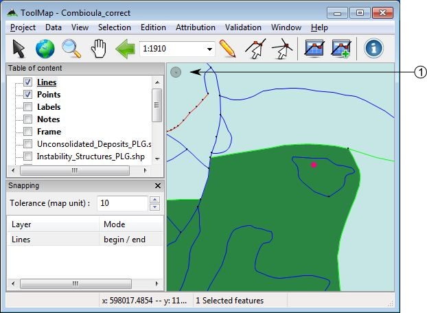
- Snapping tolerance
The options Add layer… and Remove layer… are both accessible in the menu Edition → Snapping or with the contextual menu of the snapping panel.
Attribution
The attribution function allows assigning descriptive properties to the selected feature or group of features. The descriptive properties of an object are defined by the following elements:
- The object kind
- The attributes bounded to the layer of the object
The access to the attribution functions is made with the menu Attribution
- Object Kind
- Object Attribute (single feature)… (Ctrl+A)
- Object Attribute (multiple features)… (Ctrl+Alt+A)
- Object Kind Panel
- Orientation (interactive mode) (Ctrl+Y)
- Shortcut…
Object kind
This level of attribution is made with the object kind panel. This panel can be activated with the object kind… option of the Attribution menu or by clicking on the Object Kind button in the toolbar.
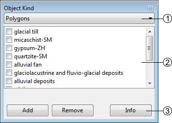
- The current construction layer in edition
- The list of objects related to the construction layer defined in (1). This list can be reordered using a contextual menu. In the line layer the objects are distributed in two categories:
- Frequent objects
- Less frequent objects.
The assignation of the object kinds to one or the other category is made at the level of the object kind definition (cf: Edit object).
- Object kind controls:
- The [Add] button allows you to add one or more object kind. It will only adjoin the selected new object(s) to the selected features without removing their previous attribution.
- The [Remove] button allows to remove one or more object kind. It will only disjoin the selected object(s) from the selected features.
- The [Info] button allows displaying the kinds attributed to the selected feature (enable only for a single selection).
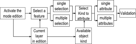
Object kind attribution scheme
Object attribute
Some layers have linked attributes, which describe the related objects. The attributes can be assigned with the Object attribute (single feature) window. This window can only be displayed when selecting an unique object. It is available through the Object Attribute (single feature)… option of the Attribution menu or by clicking on the Object Attribute button in the toolbar.
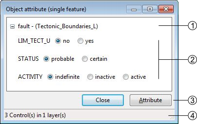
- Name of the Layer
- Attributes
- Save or Cancel the modifications
- Number of attributes available
Object attribute batch
The Object attribute(multiple features)… option from the menu Attribution allows you to assign a same attribute to all the selected features having the same object kind:
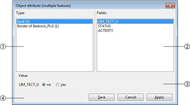
- List of the objects kind corresponding to the selected features, the value in bracket indicates the number of selected features corresponding to the same kind.
- List of the attributes corresponding to the layer of the selected object kind
- Value of the selected attribute, the value can be a text, an integer, a float, a date or an enumeration type (in this case: a text). There you can assign the new value to all the selected and concerned features. Only one attribute can be edited at once, apply your modification before making another changes.
- Attribution batch controls:
- [Save]: save the modifications and close the window
- [Cancel]: cancel the modifications and close the window
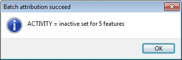
- [Apply]: apply the modifications without closing the window, a message appears to confirm the succeed of the operation.
Object Kind Panel
The object Kind Panel from the menu Attribution allows you to activate three options if checked:
- Full attribution: immediately open the advanced attribution window after the basic attribution of an object
- Empty list after attribution: automatically clear all the object kind previously selected after the attribution
- Auto display attributes: automatically display the attributes when selecting an object
Attribute orientation to point
In the case where the object can be oriented, you can give a feature an orientation. You have two ways to do it:
- From the Object attribute window, just enter the value in the proper attribute.
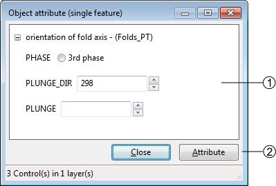
- Some text attributes (the number in bracket is the maximal number of characters, this number is defined in the attributes properties)
- The orientation attribute
- Attribution controls
- Number of attributes available
- With the option Set orientation (interactive mode) (CTRL+Y) from the menu Tools, your cursor also change and you will be able to assign an orientation with a click-and-release action.
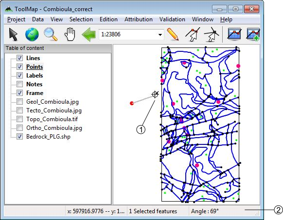
- The orientation cursor
- The orientation indicator
Once you have release the click, the value of the orientation indicator is attributed to the feature.
Shortcuts
The Shortcut… option of the attribution menu allows to assign shortcuts to facilitate the attribution.
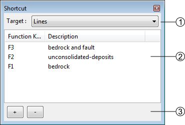
- Drop-down menu allowing to select the construction layer where the shortcuts are assigned.
- List of the shortcuts and descriptions. Following operations can be realized in the list:
- Edit the shortcuts characteristics by double-clicking on it
- Reorganize the list of shortcuts with the contextual menu by right-clicking
- List of shortcuts management controls
- [+]: add a shortcut
- [-]: delete a shortcut. The suppression can also be made with the DELETE or BACKSPACE keys.
The shortcuts edition window looks like the following:
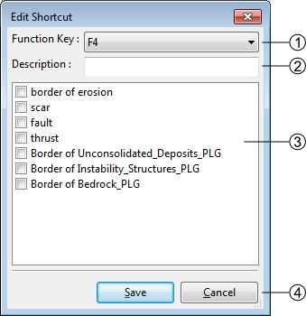
- List of key functions available which can be assigned to a shortcut
- Description of the shortcut
- Object kind associated to the shortcut, the shortcut can attribute more than one object
- Apply or Cancel the modifications
At the attribution with a shortcut, you have a message in the status bar that confirms the attribution.

Validation
The validation allows verifying the geometrical and semantic meaning of the objects. It is done with the menu Validation:
- Queries Panel
- New query
- Remove selected query
- Run selected query
- Dangling Nodes
Semantic Validation
The semantic validation of your data is made with the use of queries. The queries are available in the Queries panel. You can activate it by clicking on the Queries Panel option in the Validation menu.
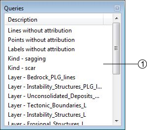
- List of available queries. Several operations are available with a contextual menu:
- Run query: run the selected query.
- Use query for symbology: directly assign the query to the multiple symbology of the correspondant layer.
- Edit query SQL: Open the Edit queries window allowing you to work on the SQL code of your query.
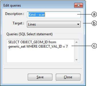
- Query description
- Construction layer on which the query will be applied
- Definition of the query in SQL language
- Add query: Display Query wizard allowing you to easily create a new query.
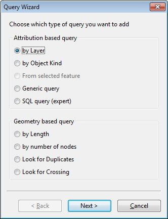
There is basically two types of queries; the attribution and the geometry based queries:
- Attribution based
Those queries look for the attribution of the features to sort them out. While the queries on the object kinds are very good to search for precise features, the queries calling the layers are often more suited to highlight the general structures.
- Geometry based
Those queries only call the structures of the features stored in the construction layers. Their main goal is to prevent the existence of unnecessary features or structural errors.
Geometrical Validation
The Validation menu includes the option Dangling Nodes… which allows to highlight the geometrical errors of the lines related to polygonal layers. The problematic nodes are identified with a red and white circle. The geometrical validation tool window looks like the following:
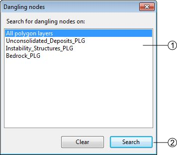
- Research extent
- [Search]: search the errors
[Clear]: clear the highlighting of the errors
There is basically two types of errors:
Dangling nodes

The polygon is not closed. This is mainly due to a bad snapping. Make sure to use the snapping panel efficiently.
Missing attribution

The nodes are correctly snapped but the segment between the highlighted nodes is badly attributed, it shall have the same object kind as the orange lines.
This is actually a semantic error, but sometimes you can miss it with the queries because of very small lines.
Redactor Mode
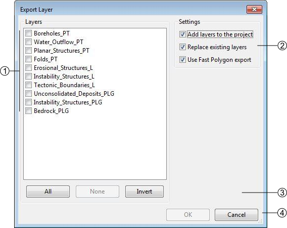
The redactor mode allows you to export your layers and reimport them into ToolMap so you can check the consistency of your data. The process is made with the Export Layer… option from the Project menu.
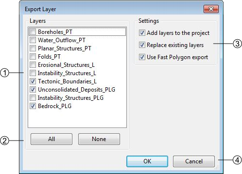
- List of all your layers, check those you want to reimport as shapefile
- Layers selection controls
- Settings
- Add layers to the project: If checked, automatically import the layer(s) into the project.
- Replace existing layers: If checked, replace the pre-existing version of the same layer.
- Use fast polygon export: If checked, …
- Validate or cancel the operation
The reimported layers will appear in the table of content as support layers. Like other layers you can access to the symbology window with the contextual menu. This window allows you to classify the different objects in your layers.
- List of auto generated filters for the classification. The layer can be classified with:
- the objects kind
- the attributes (if some)
- the number of labels lying in each polygon
- List of the generated classes depending of the selection in (1). The classes are actually generated with queries. You can modify them for improved classes.
- Symbology controls:
- Classify: Generate the classes depending of your choice in (1)
- Add: Add a new class, you will have to write the query yourself
- Remove: Remove the selected class
- Remove all: Remove all the classes
- Validate or cancel the changes
By double-clicking on a class you can edit its own symbology.
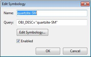
Several options can be changed:
- you can enable/disable a class by checking or not the option. The disabled classe is not displayed in the GIS Window and its name appears grayed in the symbology list.
- You can change the visual effect of your class by clicking on edit symbology; you are able to change the style, the color the width and the transparency.
Those layers can then be displayed like any other support themes.
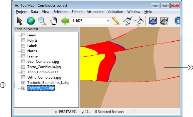
- Reimported layers
- Example of two layers with edited symbology.
The redactor mode is very usefull to sort out the labelization errors. The classification with the number of labels lying in each polygon grant you an easy view of the missing or excess labels.
Functionalities
In ToolMap you have several windows providing you some extra tools or informations. They are described below.
Preferences
The Preferences window is accessible through the menu window → preferences. It contains some basic settings accessible at any time. (even if no project is opened).
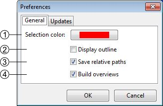
- Set de color of the selected features (red by default).
- Display a white outline around the selected features if checked.
- This option makes ToolMap remember the relative path and not the physical path of the linked data.
- This option allows toolmap to build overviews for the data which don't have them already. It can greatly improve the performences of ToolMap in the case of heavy data.
On the second tab of the window, there are the options related to the connection. If you have an access to internet ToolMap will automatically check for new updates.
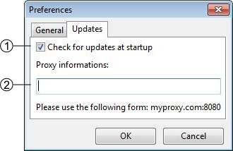
- activate/deactivate the update check
- Information to fulfill if your connection is behind a proxy
Information window
The information window is accessible with the menu window → information window. It displays informations about selected features or layer.
Feature tab
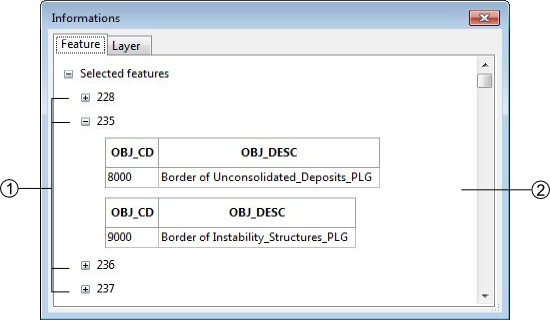
- Selected feature ID
- Features type and attributes
Right-clicking on a feature ID gives you can access to a contextual menu with the following operations:
- Move to: center the screen on the selected feature
- Zoom to: adjust the scale to display the selected feature on the whole screen (this option does not work for the point type layers).
- Remove from selection: remove a feature from your selection
- Select this feature only: unselect all the other features in your selection
- Copy data to clipboard: copy the informations of the selected feature
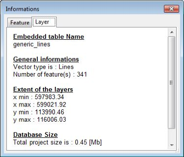
Layer tab
The Layer tab of the Information window displays all the informations on the selected layer.
Layouts
You can access ToolMap's different layouts using the Layout option of the Window menu. These allows you to use three different kinds of windows disposition:
- The Default layout, which is the one you get when first launching ToolMap. This is the one displayed in the User Interface Overview.
- The Vertical layout, which includes all the useful windows in a vertical display.
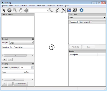
- The Horizontal layout, which includes the same windows than the Vertical layout but do so in the left border and the bottom of the display window.
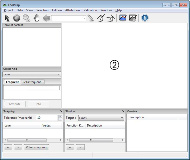
You can freely close any of the tabs you wish using the corresponding menu or reorganize your tabs by clicking and dropping them where you want them to be. ToolMap will then remember your new custom layout and display it when you launch it.
You can switch back to one of the three base layouts anytime by simply selecting them again in the Window menu.
Statistics
The statistics window is accessible with the option Statistics… of the menu Tools. It allows you when launched to count some of your editing activities.
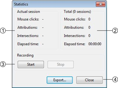
- Statistics of the current session, it displays the number of clicks made in the visualization window, the number of attribution and intersection you made (i.e. the number of time you used the function intersection or attribution, if you attribute five objects at once it is considered as one)
- The sum of all the statistics you made on this project
- Statistics management: allow you to start or stop a statistic session. Clicking on start or stop immediately close the window.
- The export option isn't available yet.
Tutorial
Welcome in the ToolMap tutorial
This part of the wiki is dedicated to help you beginning with ToolMap. By following this tutorial you should be able to:
- Understand how ToolMap works
- Define and create a project of your own
- Vectorize it properly
- Validate your work and export it
On the following pages you will have the opportunity to follow the creation of a project. You can have access to the exact same data wish you to work while reading.
Those data are accessible here : Tutorial data
Data decription
The compressed folder is constitued such as this:
- ToolMap
- 01 - Project: folder intended for the storage of the project.
- 02 - Data: folder containing .tiff files used as support data.
- 03 - Export: folder intended for the exportation of your project.
- 04 - Backups: folder intended for the backups.
- 05 - Other: folder containing the legend of the maps and the pdf of the data model such as in the tutorial.
- 06 - Templates: folder containing two tmtp files. Those files allow you to create a project from a template.
- data_model.tmtp: Project with implemented data model but no features vectorized.
- Complete.tmtp: Project fully completed.

Generalities
What is ToolMap?
ToolMap is a cost-free, open-source software dedicated for digitizing data and producing complex multi-layer GIS projects.
It was developped in response to the need to create projects with:
- A faultless and accurate topological structure.
- A correct and homogenized semantic attribution.
How does it work?
ToolMap perform its duty based on two basic and undissociable principles:
- The data model describing the nature and spatial relationships between the possible different features.
- The digitizing process allowing only two types of geometries, lines and points to represent all two-dimensional “real-world” objects. No polygon layer exists in ToolMap; they are built from the combination of lines delinaeting surfaces. Digitizing all lines, line feature (strictly speaking) and borders of polygons within one single layer yields the following advantages:
- No redundancy in the digitzing process: geometric shapes referring to multiple object types are digitized and stored only once.
- Perfect match between geometric shapes occurring in different thematic GIS layers: all objects are extracted from the same construction layers.


What is the data model?
The data model is a structure of data composed to represent the reality you want to vectorize. In the data model lay all the information you want to get at the end of your work. It sorts the data of the same nature together in layers. Seeing that fact, the more intricate a project is the more layers you shall have. Those layers may represent 3 types of geometries:
- Points
- Lines
- Polygons
Practical case
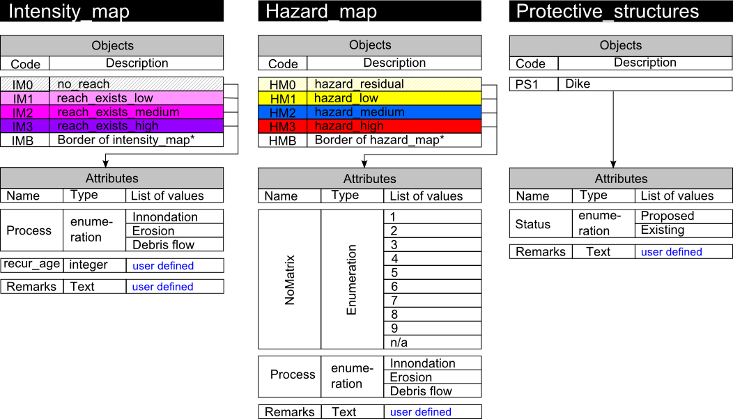
In the subsequent case you will follow the realization of a new project. It is the hazard study of an area. The goal is to digitize the data properly. After analyzing them thoughtfully you can divide them in 3 different layers:
- A line layer containing information of the protective structures.
- A polygonal layer containing information of hazards
- A polygonal layer containing information of intensities
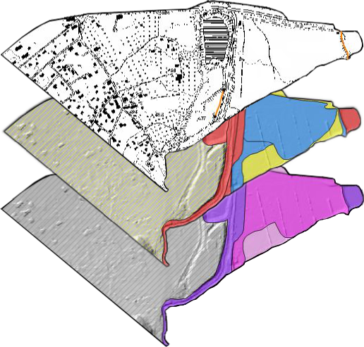
Those are the information you choose to vectorize. To do that you will need a different layer for each map; meanig two polygonal layers and a line layer. Each color of the polygonal layers represent a different object. Each object can then have individual properties. Those properties are described by the attributes. For exemple a medium hazard (object) can stem from an innondation or a Debris flow event (attributes).
All the objects can then be illustrated the following way:
Every layer is built to satisfy the necessities of the project. It means that to work with ToolMap efficiently you have to previously analyze your data to define what your final objective is so you can easily generate your data model.
Implementation in ToolMap
Once your data model is defined, meaning it describes adequatly all the data you want to digitize, you will have to implement it into a ToolMap project. Launch ToolMap for getting started.
First of all you need to create a new empty project.
Project → New project → Empty...
After clicking on the [Create new project] button the Project definition window pops up. On the Project properties tab set the name of the author and some comments if wanted.
The spatial model tab allows you to implement your data model. It lists all the layers defined in your project. At this particular moment it is empty, but you will fulfill it with the layers you imagined as your data model.
Click now on the [+] button to add your first layer…
The Thematic layer definition window pops up. You will have several operations to do:
- Set the name of your layer
- Define its geometrical nature
- Create the objects contained in this layer
- Create the attributes characterizing the objects
The objects are listed on the first tab of the window. Click on the [+] to create a new object. Set a code and a name for every object.
The attributes are listed on the second tab of the window. Click on the [+] button to create a new attribute. Every attribute is defined by a name and a type. In this case we have 3 different types:
- Enumeration: the list must be computed. Each input is defined by a code and a name.
- Integer
- Text: the number of max characters must be defined.
Once you computed every information click on [Ok] to validate your layer and go back to the Project definition window. Create, following the same process, every other layers needed.
After your data model is fully implemented. Finish the creation of your project by clicking on the [Save] button.
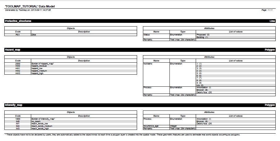
Data model overview
At any time (after the creation) you can export the model of your project as a pdf file.
Project → Export Model as PDF...
The Export data model layout window allows you to choose between some display options, let the default display for the time being. Finalize the export by choosing a path to save the pdf file. If you followed rigorously the tutorial you should have something like:
Vectorization
The digitizing process goes through the vectorization of the following layers:
- Frame (line)
- Points (point)
- Lines (line)
- Labels (point)
Those layers are displayed in bold in the table of content.
Getting ready
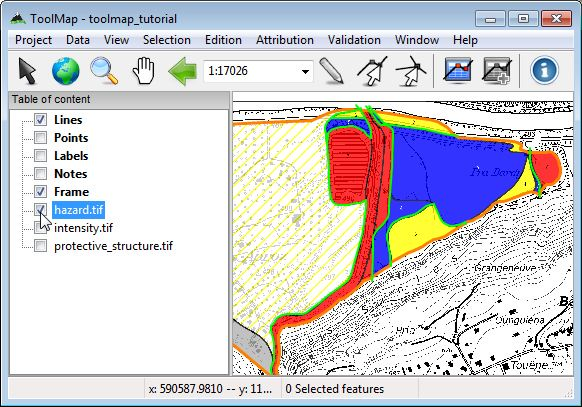
Link data
Your project is now opened, but you will need some support themes as reference and base of vectorization.
Data → Link data... (Ctrl+O)
Navigate to ToolMap → 02 - data, select all the files and click on [Open]. The linked files now appear in the table of content.
Activate snapping
The snapping option allows you to be certain two vertices are indeed at the exact same location.
Edition → Snapping → Snapping panel... (Ctrl+G)
By right-clicking on the panel display the contextual menu allowing you to add a new layer to be considered for the snapping. Display the layers Lines and Frame
Set the tolerance to 6 (depending your preferences and at which scale you are working you may want to increase/decrease this value).
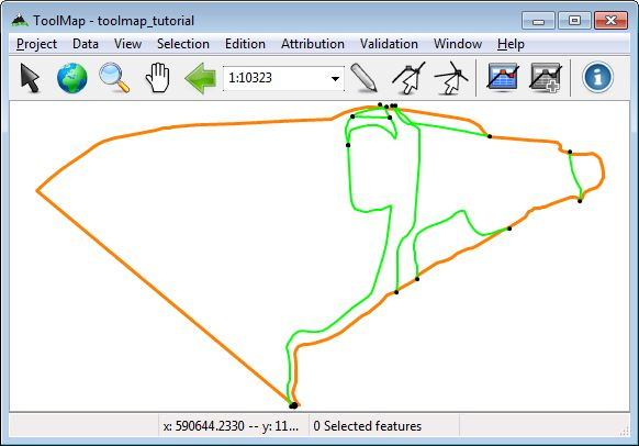
Draw the frame
Now that the snapping is set, define the area of study by drawing the frame.
Right-click on Frame → Edit layer
The layer is now underlined in the table of content meaning it is in edition. By selecting the draw tool start vectorizing the frame.
Edition → Draw feature (D)
Draw the frame by creating vertices all around the desired zone. Once at the end, put your last vertex a bit on the side and validate the frame with the [Enter] or [Tab] key. The vectorized line may not be very visible, to solve this little issue change the symbology of the frame.
Right-click on frame → Symbology
Change the color for orange (or any visible color) and set the width to 3.
You now have to close properly your frame:
Edition → Modify feature (M)
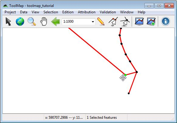
Click on the last vertex and drag it near the first vertex, if the snapping is set correctly it shall be attracted to it ensuring the geometrical validity (vertex displayed in green if it is the case). Finish the modification by clicking on the [Enter] key.
Drawing the lines
Settings
There are some few things to set before truly starting to vectorize the lines:
- Right-click on Lines → Symbology
Set the color to a nice flashy green and the width at 2.
- Right-click on Lines → Show vertex → begin/end
This will display the vertices on both sides of every line. This will help a lot to know where you will be able to snap your lines.
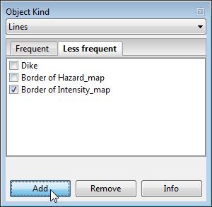
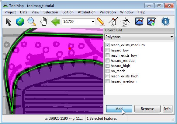
- Attribution → Object kind...
Open the Object kind panel where all the objects of the project are listed and sorted by layer type.
- Uncheck all the support files but “Intensity_map” in the table of content.
You will use the others after finishing the vectorization of this map.
Edition/Attribution
The line creation is a 3 steps process:
- Vectorization
- Object definition
- Object attribution (if available)
Remember that every segment of line can be attributed differently depending upon the other levels of information. So every time you encounter an intersection you will have to undergo the 3 steps process.
Like we did for the frame, we have to enter the edition mode on the Lines layer this time.
Right-click on Lines → Edit layer
1. Edition → Draw feature (D)
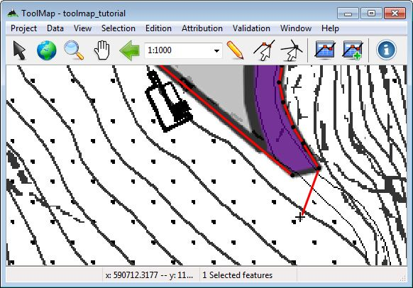
Draw your first line until you find an intersection. Validate it by clicking on the [Enter] key. For the lines starting/ending at the frame don't be afraid to draw them out of it. They will be cut on the export anyway.
The created line is automatically selected after validation. By default the selected lines appear in red, all their vertices are also visible. When editing the Lines layer the line objects are automatically displayed in the Object kind panel.
2. Check Border of Intensity_map → press [Add] button
3. Attribution → Object attribute (single feature)... (Ctrl+A)
Nothing happens, your object “Border of Intensity_map” is a line delineating a polygon. It has consequently no attributes.
The 3 steps process is now finished, reiterate it for the rest of the lines. The frame act as a border of polygons, so don't bother vectorizing lines on it to close your polygons. Finally your project should start to look like the following:
Drawing the labels
At this stage the lines delineating the borders of the polygons of the intensity_map layer are drawn. But they are actually only empty surfaces. To give them their descriptive object and attributes you have to edit the labels. The process is similar to the lines but somehow more simple.
Settings
Right-click on Labels → Symbology…
Set the color a nice light blue and the radius at 8
Edition/attribution
Right-click on Labels → Edit layer
The labels don't have any topological meaning. It is why the exact location of your labels is not important. The relevant thing is to have one label laying within the borders of every polygonal surface you want to digitize.
1. Edition → Draw feature (D)
As the labels are point type geometries it is quiet easy to draw them. Click on the wanted location and the label is already created. There is no need to press a finalizing key like for the lines. Once it is created it is automatically selected and ready to be attributed.
2. Check appropriate object → [Add]
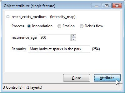
3. Attribution → Object attribute (single feature)… (Ctrl+A)
The Object attribute (single feature) window pops up. Set process to innondation, recurrence_age to 300 and you have the liberty to write a comment if you desire.
Reiterate the process as many time as needed to put one label in every surface appearing on your Intensity_map. You should slowly get to a map such as this one:
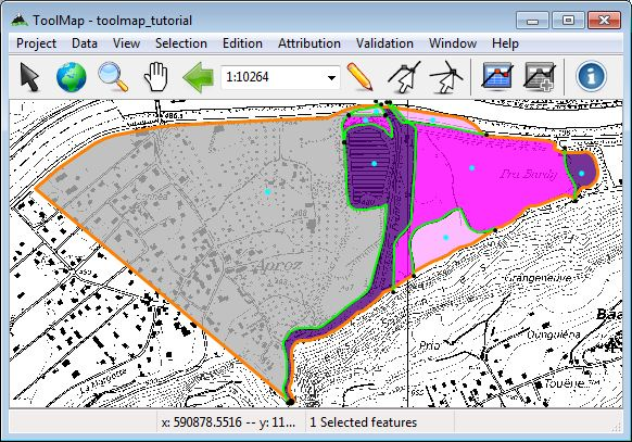
Move from one support to another
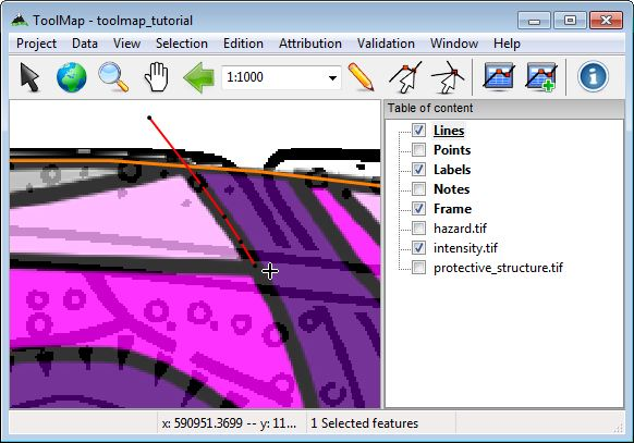
Until now you went through the vectorization of one support theme but there is still plenty information to digitize. Change the display of the support themes. move from Intensity_map to Hazard_map.
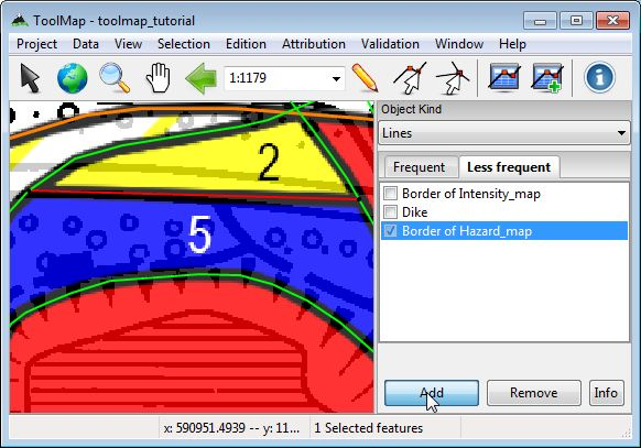
As you can see on the picture above, a lot of structures are actually redundancies of what you already vectorized. The lines consistent with the new support theme have to be attributed as part of this layer.
Right-click on Lines → Edit layer
Edition → Select feature (V) → [Add] new attribution
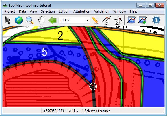
Once you have attributed the existing lines, you have to draw and attribute the rest of them. On this map there are new intersections. For that purpose create them by cutting the existing lines. The tool cut line allows you to cut a line on an existing vertex. The cutted line will be divided at the location of the vertex. If there isn't a vertex at the desired location, you can easily add one with the insert vertex tool.
Optional: Select a line → Edition → Insert vertex (I)
Select a line → Edition → Cut line (Ctrl+X)
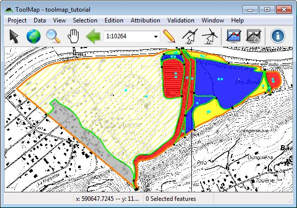
When you are finished with the vectorization/attribution of the lines, reiterate the operations of the chapter ”Drawing the labels”. At the end you shall have something looking like this:
Move on
There is still the last layer to vectorize and attribute, the instability structures. As it is a line layer you just have to follow the process of the chapter ”Drawing the lines”.
Hint: No vectorization should be required ;)
In this exemple each support theme represent a different layer. It is however possible to have more complex maps with more information on it. The processes remain the same you just have to mix them.
Validation
After the vectorization phase comes the validation. You don't want to export layers with wrong attributions or topological errors. hopefully there are strong tools to check up your work in ToolMap.
Polygons structure
You have to make sure your borders of polygon delineate correctly all your surfaces. If they don't you will have problems at the export.
Validation → Dangling nodes → Intensity_map
If the tool finds dangling nodes it means that at least one surface is badly closed. If it is the case, correct your error either by snapping the lines properly or attributing them adequately.
Reiterate this operation for the Hazard_map layer as well.
Attribution
Sadly ToolMap can't yet prevent the human factor. So if you misattributed a feature, it won't be automatically corrected. To identify those mistakes use the queries. Using the query wizard create a query for every object.
Validation → New query...
The queries can be used to apply a different symbology on two groups of features. Use this option to sort your data and eventually discover mistakes.
right-click on a query → Use Query for symbology
or
right-click on current layer → Symbology… → Multiple symbology

Map with highlighted features of the Intensity_map layer
Export
At this stage the only thing left to do is to export your layers. You will need to define the export path of your project for that.
Project → Edit → Settings... → Export path
Set the export path, you can use the folder “03 - Export”. You are now ready to export your layers.
Project → Export layer... (Ctrl+Alt+E) → [All] → [Ok]

You can now use your shapefiles in other softwares. See below the attribute table of my Hazard_map shapefile in Qgis for exemple:

Thanks
Thank you for following this tutorial, we hope it provided you the help you needed to start with ToolMap. Find out more advanced tips on the vectorization, attribution and validation process further in this Wiki.
Tips
Tips
Welcome to this part of the wiki. Before going further be aware that the following topics may require a good understanding/ knowledge of ToolMap but can eventually help you use it with more ease.
The strategies described are not by any means mandatory to use. They are just some observations made on a frequent use of the software. They browse the three main domains of ToolMap:
While looking through the following pages, you may reach to the conclusion that most of those tips are interlocked. This is due to the fact that the vectorization, attribution and even the verification are finally all part of the same edition process. Prompted by this knowledge, the ultimate handling of ToolMap would be to conjugate the different stages of the creation into one unique fluid motion.
Obviously this “motion” will variate on a case-by-case basis according the structure of the project and your preferences. In the end, the main objective would be for you to develop your own working process which fits you the best.
Advanced Vectorization
This topic relate all the strategies concerning the vectorization.
Homogenized drawing
If you want your final results to be consistent you should allways draw your lines at the same scale. In addition, to get smooth results your drawing scale shall be at least 10 time bigger as the original map. By doing so you will see nice and round lines instead of sharp edged segmented ones.
exemple: for a 1:10'000 map digitize your lines at a 1:1'000 scale
Clean intersections
When having a enormous project, the number of intersections increase fearsomely. It would be better to have a way to draw them properly without worries. For that purpose the tool Create intersection is really handy.
Start with the drawing of the biggest structures and vectorize them without interruption. By proceding like that you insure the clearness of those lines. I would either recommand to directly attribute those lines.
As you can see on the picture above, there is a lot of intersections totally ignored. Now draw the smaller features the same way you would do near the frame (i.e. wider than needed) and directly attribute them. Then:
⇒ Ctrl+I: It automatically creates the intersections and cut the lines.
⇒ Shift + select: Unselect the part you want to keep.
Now your selection is composed only by two superfluous lines you can delete.
As a result you have:
- Two intersections with very continuous lines on every sides.
- Insurance there isn't any snapping issues.
- Lesser segments to attribute.
Just make sure to add a new attribution on the newly created segments if needed.
Attribution
This topic relate all the strategies concerning the attribution issues.
Shortcuts
This change of approach makes the use of the shortcuts much more versatile. Previously you had to anticipate the features with multiple objects to create the appropriate shortcuts. While now, the shortcuts will only add their object(s) to the selected feature(s) giving you a greater liberty of use. They can also be used in series, if you hit three different shortcuts on the same selection it will recieve all the attributes defines by the shortcuts.
How and how much shortcuts you create shall be really dependent of your vectorization style, but it is hardly a lost of time to create a few on the most current objects.
Batch attribution
In the case you have a large quantity of small features which have attributes, it can be humdrum to do it one after the other. To prevent such boring work, you can select all the features with the same characteristics to attribute them at the same time using the option Object attribute (multiple feature)... (Ctrl+Alt+A).
You could differenciate two possible cases where this option could become very profitable:
- You have some features, the characteristics are the same for all of them: Select all the features using a query and attribute them.
- You have a lot of features, the biggest part of them have the same characteristics: Select all the features and give them the most usual attributes. Rework afterward the few having a different attribution.
FAQ
Rotation Warning
Introduction
Some raster files have associated rotation information. This indicates that an appropriated rotation should be applied for the raster to be correctly displayed. ToolMap display a Warning when such files are encountered because displaying those files with rotations isn’t supported yet.
To still use those images we need to convert them into non-rotated raster. Following method may be used for that purpose:
 Rotated raster. 2)Exported non rotated raster")
Using ArcGIS
- Load the raster
- Right-click the raster name in the Table of contents
- Choose Data → Export Data
- Select the Location, file Format and file name
- Press Save
The new raster is now correct and didn’t contain anymore rotation information

Note about word files (tfw)
Since ArcGIS 9.2 no more word files (tfw) are written and the georeferencing information is now stored in a aux.xml file(see ESRI help: http://tinyurl.com/68ykjqu). It is however possible to manually create such word file using “Export Raster Word File” tool from the ArcToolBox
